Key Terms

o       Distribution

o       Probability function

o       Probability density

o       Expectation

Objectives

o       Recognize a distribution and its relationship to statistics and probability

o       Distinguish between discrete and continuous distributions

o       Calculate the mean and standard deviation of a distribution

Continuous and Discrete Distributions

Statistical distributions can be either continuous or discrete; that is, the probability function f(x) may be defined for a continuous range (or set of ranges) of values or for a discrete set of values. Below are two similar distributions for a random variable X; the left-hand distribution is continuous, and the right-hand distribution is descrete.

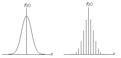
As it turns out, a probability in the case of a discrete distribution is defined as the value f(x_i), where x_i is a potential values of the random variable X. The sum of all the probabilities f(x_i) is unity (recall that the sum of all relative frequencies of a statistical data set is unity). The probability in the case of a continuous distribution is not so simple. Recall from real number theory that there are an infinite number of values between any two real numbers--thus, if we simply said that the probability of a particular value x for random variable X is f(x) (called a probability density), then the sum of the probabilities for all possible outcomes would be much greater than unity. However, this situation is not allowed. The probability that a random experiment produces an outcome from the sample space is unity. Instead, a probability for a continuous distribution is defined only for ranges of values--for instance, c < X ≤ d. The probability in this case is actually the area under the curve for c < x ≤ d, a problem which (generally) requires integral calculus to solve. Thus, the total area under the curve of a continuous probability distribution is unity. For certain distributions, easily accessible tables of values provide us with probabilities for certain ranges of values given particular continuous distributions. For the remainder of this article, however, we will focus primarily on discrete distributions.

In addition to the probability function f(x), we can also define a similar function that relates probability to the cumulative relative frequency. Recall that the cumulative relative frequency for a particular value x is simply the sum of the relative frequencies for all values less than or equal to x. If we call this function F(x), then F(x) is equal to the probability that X ≤ x for some value x. Symbolically,

F(x) = P(X ≤ x)

Mean and Variance of a Discrete Distribution

We have already studied how to calculate the mean and variance (and therefore standard deviation) of a set of statistical data. How do we go about this calculation for a distribution? The same concepts apply; a distribution is simply another way of expressing a set of statistical data. Thus, given a discrete distribution for random variable X, we can calculate the mean μ (also called the expectation--or mathematical expectation--of X) of the distribution using the following formula.

This formula simply states that the mean is the sum of the products of all values x_j in the sample space and their relative frequencies f(x_j). In this notation, j is simply an index that spans all possible values of the random variable. Note that we do not divide by a total number of values, because the relative frequency already incorporates this operation. We can illustrate the use of this formula by way of a practice problem.

Practice Problem: A player is rolling a "fair" six-sided die (each number, one through six, has an equal probability of turning up in a given roll). What is the expectation of a single roll?

Solution: Each outcome, {1, 2, 3, 4, 5, 6}, has an equal probability of 1/6 (since there are six possible outcomes). Thus, the relative frequency of each number on the die is 1/6, and the function f(x_i) = 1/6 for all values x_i. We can calculate the expectation μ of a roll (that is, of the probability distribution) using the formula above.

Note that 3.5 is halfway between the outcomes 1 and 6. This is the expectation (or mean) of the roll.

We can also calculate the variance σ² of a random variable using the same general approach. Note, based on the formula below, that the variance is the same as the expectation of (X – μ)².

As before, we can also calculate the standard deviation σ according to the usual formula.

Practice Problem: What is the standard deviation of the roll of a fair die?

Solution: Recall the distribution information from the previous problem. We first must calculate the variance of the distribution.

The standard deviation is then

Practice Problem: A scientist is collecting measurement data for a certain system parameter. His data include the values {1.23, 1.29, 1.37, 1.84, 1.18, 1.22, 1.25} with associated frequencies {3, 5, 4, 1, 6, 2, 4}. Based on this information, estimate the expectation of the next measurement.

Solution: The problem asks us to calculate the expectation of the next measurement, which is simply the mean of the associated probability distribution. The set of relative frequencies--or probabilities--is simply the set of frequencies divided by the total number of values, 25. This set (in order) is {0.12, 0.2, 0.16, 0.04, 0.24, 0.08, 0.16}. Now, let's calculate an estimate for the expectation of the next measurement. (Note that we are using a sample--we do not have all the data for all possible measurements. Thus, this result is only an estimate of the expectation, because the "true" probability distribution cannot be determined for certain.)

Thus, the mean of the distribution is approximately 1.28. Note that the expectation (mean) of the measurement is not necessarily the most likely outcome, nor is it necessarily the particular value that the scientist should expect to see in his next measurement. It is, however, what the scientist should expect for a mean (average) of a series of measurements.